Programming-free Image-Analysis Workflows for IHC, IF and Spatial Proteomics: More than just Cell Counting
DOI: https://doi.org/10.47184/tp.2024.01.06Quantitative analysis of cells using a specific protein marker is one of the most frequently performed tasks in both preclinical and clinical histopathology. The primary alternatives include immunohistochemistry and immunofluorescence. This article will briefly shed some light on the pros and cons of both methods, the main ones being that immunohistochemistry is widely available, but in many laboratories, it is limited to only one marker per image. Utilizing more than one marker can be achieved through methods such as establishing duplex or triplex stains, serial sections, or re-staining. However, immunofluorescence excels where a deep multi-marker characterization of single cells is required. Spatial proteomics systems have recently increased the plexity to as many as 100 parallel markers, allowing advanced co-expression, rare cells, and spatial neighbourhood analyses. Bioinformatic analysis aspects for both modalities are discussed, outlining two generic workflows as they are realised in a professional image analysis software used by biomedical researchers. While cell segmentation and typing are at the core, a number of pre- and post-processing steps, such as tissue detection, comparison of ROIs, hotspot search, spatial clustering or neighbourhood analysis should be performed to provide more comprehensive read-outs.
Keywords: Digital pathology, spatial proteomics, image analysis, IHC, IF
Pros and Cons of IHC vs. IF
Immunohistochemistry (IHC) – A clear advantage of IHC is that it is readily available in almost all pathology institutes and does not require a dark laboratory setup or a housed microscope. After staining, the targeted cells appear in a specific colour when viewed under a brightfield microscope, typically brown or red depending on the chromogen used, while the remaining cells are made visible using a counterstain, typically blueish haematoxylin. While duplex or even triplex IHC is possible, its use has remained somewhat exotic. Instead, when multiple markers are desired, consecutive (“serial”) sections are sliced from a single tissue block and in each section a different antigen is marked. The limitation of this workaround is evident. More tissue is consumed, the amount of glass slides to be evaluated (and scanned) increases and tissue sections have to be aligned to one another when local co-occurrence is of interest. The co-localisation of multiple antigens in the same cell is barely detectable because a particular cell visible in one section is not visible in all remaining tissue sections, oftentimes not even in an adjacent section. This problem can be mitigated by establishing a co-staining protocol in which a single tissue section is subjected to multiple cycles of staining, scanning, washing. However, only very few pathology laboratories employ co-staining in their research, and the amount and order in which stains can be applied is limited.
Immunofluorescence (IF) – On the contrary, the significant strength of immunofluorescence lies in its easy capability to analyze the co-localization of proteins. Here, multiple antibodies are frequently applied in parallel and different fluorescent dyes piggyback on these antibodies. By coupling specific antibodies with dyes of different wavelengths, multiple proteins can be visualised at the same time on the same tissue. The number of parallel dyes is limited by the availability of (affordable) narrow-band optical filters that let only the light emitted by a particular fluorescent dye pass. However, under the umbrella headline spatial biology, which also includes spatial transcriptomics and other *omics methods, several vendors have developed technologies for spatial proteomics in recent years that allow driving the number of simultaneously detected proteins up (“higher plexity”). Most vendors can be grouped into one of two technological approaches: cyclic restaining (e. g. Akoya Biosciences’s PhenoCycler, Lunaphore’s Comet, Miltenyi Biotec’s MACSima or Canopy Biosciences’ CellScape) or time-of-flight (ToF) mass spectrometry (e. g. Standard Biotools’ Hyperion, Ionpath’s MIBIscope).
Figure 1 shows the quantitative analysis workflows for IHC and IF cohorts as they are available in the MIKAIA®1 whole-slide-image analysis platform.
1 www.mikaia.ai
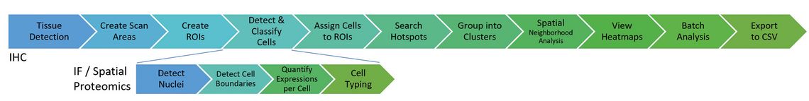
Figure 1: Analysis workflow for IHC and IF whole-slide-images as realized in the MIKAIA® studio software.
Importantly, no programming skills are needed, allowing biomedical researchers who are less interested in bioinformatics to handle computational pathology tasks themselves. Predominantly, the same preprocessing and postprocessing steps are applicable to both IHC and IF. Only the core part of cell segmentation and characterization differs, with IF providing a more accurate cell typing.
Image analysis workflow for IHC: Essentially, the quantitative analysis of IHC slides revolves around cell counting. The era of manual cell counting is far behind us. Image analysis solutions will typically first unmix both stain components, e. g. H and DAB, then detect cells in both stain components individually or in combination and finally classify them as “positive” or “negative” (or low / medium / strong), depending on the chromogen intensity. The most widely used free tool to do this is QuPath. But many studies require a more extensive analysis, and a cohort of hundreds of scans, not just of a single image, without having to program scripts.
The first pre-processing step is to detect and outline the tissue in the scanned image. This is required to normalise the cell abundance by the tissue area (in mm²) – and to avoid wasting time on cell detection in parts of the scan that contain only background.
A common additional requirement is to compare cell statistics in different regions in the tissue, such as inside vs. outside a tumor. Such a region of interest (ROI) can be manually drawn or can be generated by another image analysis module such as the MIKAIA® AI Author. Detected immune cells are then assigned to the ROI in which they are located. The remaining tissue implicitly yields the “rest” ROI. According to the enclosing ROI, detected cells are labeled in different classes such as “CD8+ in tumor” and “CD8+ in rest”. When exporting analysis results into a CSV spreadsheet that can be opened in Microsoft Excel or imported with Python, Matlab or R, both the cell abundance per ROI and the ROIs total area in mm² will be available, yielding separate cell densities (in cells/mm²). Another insightful type of ROI are concentric distance margins. Having selected a base annotation, both inwards and outwards margins of a given diameter in µm can be generated. By selecting these margins as ROIs in the IHC cell analysis, the immune density as a function of the distance from the tumor invasive front can be measured.
Another trivial, but yet critical processing step is to support the collection of separate statistics for multiple tissue specimen on the same glass slide. Users often place multiple tissue specimens onto the same slide to save processing and scanning time. In combination with ROIs, detected cells are organized in a hierarchy: a cell is located in a ROI, which is located in a tissue specimen, which in turn is located on a glass slide, which is part of a study cohort.
»Interpret cells as subway stations in a metro map«
The manner in which cells disperse within a tissue could be relevant to a biomarker. MIKAIA® provides three downstream analyses to investigate how cells are spatially organised: (1) Hotspot search, (2) spatial clustering and (3) neighbourhood analysis (also known as cell-cell-connections analysis).
A hotspot search can be employed in two different ways. In one scenario, the density of cells in the top N hotspots may be of interest, whereas in other cases the abundance of hotspots in the slide may be more informative.
The Spatial Clustering App assigns detected cells into clusters. In contrast to a hotspot, a cluster can have a dynamic size (see yellow clusters in Figure 2).
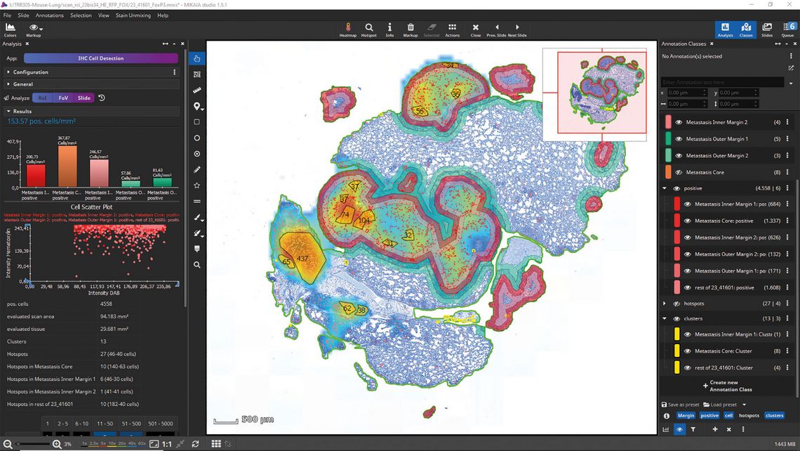
Figure 2: FoxP3+ cells in lung tissue are detected with MIKAIA's IHC Cell Detection App. Cells (red) are assigned to different regions and clustered (yellow). Slide courtesy of Univ. Regensburg, as part of DFG-funded TRR305.
It can be defined by the maximum distance between two cells: Starting with any positive cell, all nearby cells are assigned to the same cluster, and then all cells adjacent to those cells are also added to the same cluster, and so on, until there are no more nearby cells. When ROIs are involved, a cluster can be selected to comprise only cells from a single ROI or from multiple ROIs.
Finally, the Cell-Cell-Connections App interprets cells as subway stations in a complex metro map or as nodes in a graph. The app generates connections between any two adjacent cells and assigns them into different classes, depending on which two cell types are connected. This data enables a bystander analysis which states how many neighbours a cell type has on average. In addition, the cell graph also shows the average distance in µm between any two cell types.
»No biologist can resist the urge to manually correct falsely detected cells«
All of these downstream analyses rely on a robustly detected set of cells. Irrespective of the algorithm utilized, numerous IHC slides will include challenging areas with stained objects that might be misinterpreted as positive cells. Despite whether a few falsely detected or missed cells truly influence the overall narrative derived from a slide or cohort analysis, it's remarkable how almost no biologist can resist the temptation to manually correct these misidentified cells. The initial attempt will involve filtering out false positives by assessing cell attributes such as size or stain intensity. Additionally, detected cell annotations can be manually deleted and missing ones can be added. Finally, problematic regions can be marked with an “ignore” annotation.
Image analysis workflow for IF: In principle, the workflow for analysing IF slides is very similar. Pre-processing steps are tissue detection and optionally, ROI detection. ROI masks can optionally be generated by thresholding a fluorescence channel – or a combination of multiple channels – with the Mask by Color App.
A difference to the IHC analysis is that no unmixing is required, as fluorescent dyes are imaged separately into distinct color channels from the outset. Typically, the DAPI channel, which shows DNA. serves as a marker that is positive in all cells. Nuclei are detected, for instance using the CellPose AI, and then expanded by a few microns to approximate the cell boundary. When a membrane marker is present, it can be utilized to capture the cell outline more accurately.
Subsequently, each cell is assessed by measuring the mean fluorescence intensity (MFI) for each protein marker, separately in the nucleus and cytoplasm. Now, cell typing can be performed. When only a few markers are used, a straightforward approach is to configure an intensity threshold for each marker and determine for each cell whether the marker is expressed or not (e. g. CD8+ vs CD8-). Optionally, an additional constraint can be applied, requiring a minimum area to adequately express the marker. When the markers mode is selected, MIKAIA® will generate a cell annotation for each marker expressed by a cell. Annotation classes are named according to the marker. A cell that expresses both CD8 and CD3 will then result in two annotations, “CD8+” and “CD3+”. However, when the marker combinations mode is selected, each cell will only yield a single annotation. Annotation classes then refer to a specific combination, such as “A (CD8+, CD3+)”. Be cautious: when the plexity is high, the number of possible permutations increases dramatically. Next, a third mode, titled cluster, is particularly useful, where cells are not classified based on user-defined per-marker expression thresholds but on unsupervised clustering of the colour and morphometric features collected per cell. Two types of clustering methods are prevalent: either the user must pre-select the number of cluster (e. g., k-means) or the cluster variance is specified, and then the number of clusters is dynamic (e. g., DBSCAN). In fact, regardless of which of the three modes is selected, the underlying image analysis remains identical. MIKAIA® supports all three modes in a single analysis run.
IF and spatial proteomics: »A lot more insightful«
The spatial analysis with the Cell-Cell-Connections App is significantly more powerful and insightful compared to IHC, as an IF assay not only yields “positive” vs. “negative” but also enables a much more comprehensive characterisation of cells, resulting in a greater variety of cell types. The distribution of certain cell types or even cell-cell-connection types can be visualized using an interactively configurable density heatmap overlay. In the end, it may even be helpful to hide the actual image and visualize only the annotations (Figure 3).
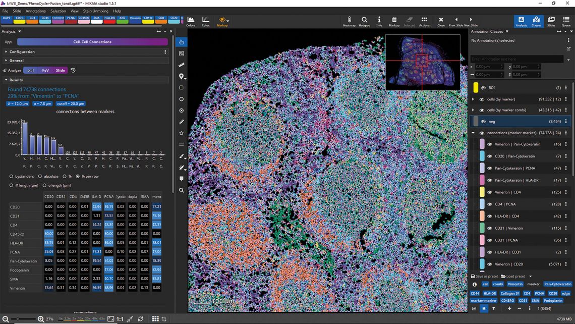
Figure 3: Analysis of 16-plex tonsil with MIKAIA‘s FL Cell Analysis and Cell-Cell-Connection Apps. Each color represents a marker-combination. Lines connect neighboring cells. Scan courtesy of Akoya Biosciences.
In conclusion, MIKAIA® offers comprehensive, programming-free off-the-shelf batch analysis workflows for both IHC and IF. While IF provides a more in-depth characterization of cells, it is less readily available in laboratories. Devices capable of high-plex IF are expensive but map the biological environment much more accurately compared low-plex IF or IHC. High-end labs should establish both methods and use IHC when appropriate and mIF when required. Considering the time and cost of sample preparation and scanning, a robust bioinformatics analysis should be conducted that yields numerous quantitative endpoints.